Benchmarking KùzuDB vs. Neo4j on a social network dataset Link to heading
Embedded databases have been experiencing something of a renaissance lately. In the first post in this series, I gave a detailed overview of this fascinating landscape, breaking it down into domains. This second post goes deeper into the graph domain – in particular, KùzuDB, a modern, lightweight, blazing fast embedded graph database written in C++ that’s emerging as a powerful option for analytically querying very large graphs.
Because it’s hard to gauge performance in isolation, I felt it made sense to run a benchmark study with respect to Neo4j, the most popular graph database in the market. The case study involves querying an artificial social network dataset that’s hand-constructed to possess interesting graph structures, while also being large enough to measure performance in a meaningful manner.
What makes Kùzu different? Link to heading
Having been a graph data scientist and practitioner for a few years now, I can say I’ve experimented with my fair share of options. The standout feature of Kùzu that sets it apart from all the others is, of course, its embedded architecture – Kùzu is natively designed to run in-process, tightly integrated with the application code written in your language of choice. In their blog post outlining their vision1, the makers of Kùzu very explicitly state their goal of replicating in the graph world what DuckDB has done for relational DBs.
In my opinion, there are a few other design decisions of Kùzu that make it particularly interesting and useful for a wide variety of practitioners.
- First-class support for the labelled property graph (LPG) model, which was popularized by Neo4j and is now more or less the de-facto standard for graph databases in industry.
- However, this doesn’t mean that RDF graphs are not supported – this is ongoing work and is part of the Kùzu roadmap2.
- Embracing openCypher as its query language, which is the most widely adopted, fully-specified, declarative and open graph query language.
- One of the main focuses of Kùzu is to achieve near-full feature parity with Neo4j’s implementation of Cypher, and the current version of Kùzu is already quite close to this goal.
- Built for vectorized execution of OLAP-type queries, which means that Kùzu is optimized for running expensive, multi-hop queries on very large graphs.
- Designed to be the storage layer of choice for graph machine learning applications, with a high degree of interoperability with geometric deep learning frameworks like PyG and DGL, as well as graph analytics frameworks like NetworkX.
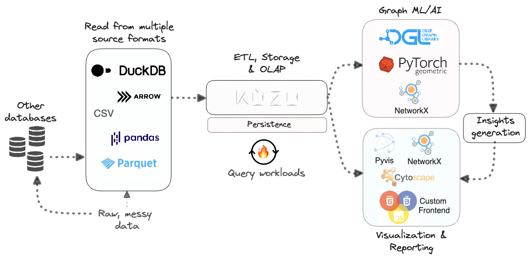
Where KùzuDB sits in the graph analytics value chain
Dataset Link to heading
Graph databases, and graph data structures in general, are ideally suited to analyze highly-connected data like social networks or financial transactions. If done in a relational (SQL) database, this could involve expensive or recursive joins on numerous data points that may have many-to-many relationships.
The artificial dataset used in this study contains data for 100,000 persons that “follow” each other, with roughly 2.4 million edges between them, as well as their interests and the locations in which they live. To keep things simple, only three countries and their cities are in the dataset – United States 🇺🇸, United Kingdom 🇬🇧 and Canada 🇨🇦. The schema for this graph is shown below.
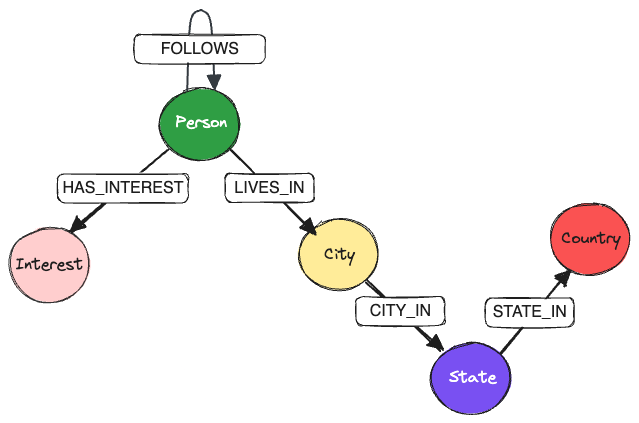
PersonnodeFOLLOWSanotherPersonnodePersonnodeLIVES_INaCitynodePersonnodeHAS_INTERESTtowards anInterestnodeCitynode isCITY_INaStatenodeStatenode isSTATE_INaCountrynode
To make the graph more interesting, a small subset (~0.5%) of the Person nodes are considered “hubs”, i.e., they are connected to up to 5% of all the other persons in the graph. This is to simulate the fact that in real-world social networks, there’s a small fraction of people who are very well-connected and have a large number of followers.
As a result, the generated graph between persons has some interesting structures, like cliques, trees and cycles, and is visualized below.
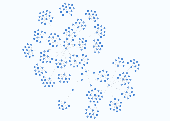
Cliques, trees and cycles in the graph of connected persons
A detailed explanation on the dataset generation is shown in the GitHub repo. Note that the data is generated using a fixed random seed, so it is fully reproducible, and the number of artificial nodes and edges generated can be scaled up or down, reproducibly, as needed.
Data ingestion Link to heading
The data for the artificially generated nodes and edges are saves to parquet format, transformed to a list of dictionaries in Python, and ingested to either DB.
- Data is ingested to Neo4j via the async API of the Neo4j Python client.
- Best practices as per the Neo4j docs for data ingestion via Python are followed, such as setting uniqueness constraints on node IDs, and using
UNWINDto ingest data in batches.
- Best practices as per the Neo4j docs for data ingestion via Python are followed, such as setting uniqueness constraints on node IDs, and using
- Kùzu, being an embedded database, comes with a Python API that can be accessed by simply using
pip install kuzu, and ingested directly from parquet via its bulk loader.
The code for data ingestion is in the files build_graph.py in either directory of the GitHub repo.
Performance Link to heading
In total, ~100K nodes and ~2.5 million edges are ingested ~18x faster in KùzuDB than in Neo4j.
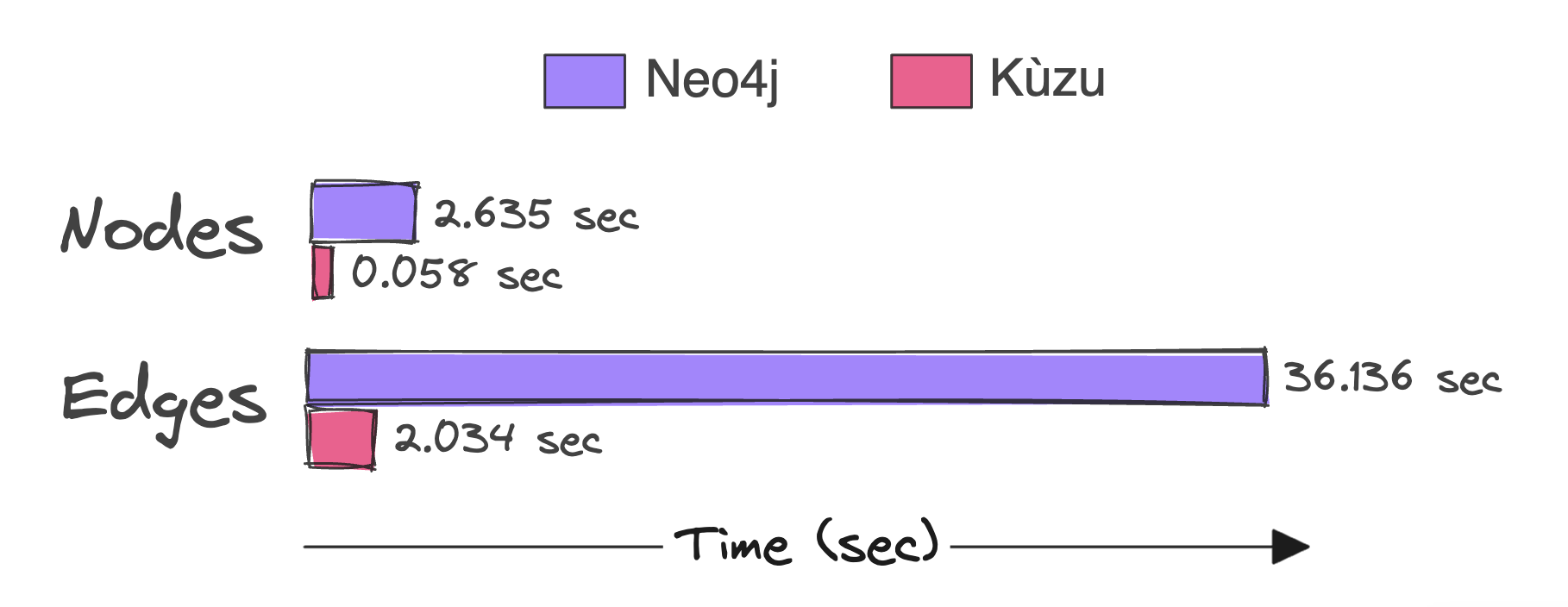
When ingesting data via their Python clients, Kùzu is ~18x faster than Neo4j for this dataset
apoc.periodic.iterate, using the Java API, or the neo4j-admin import tool, but these methods require CSV as the input format, and would also need glue code to integrate the data loading with an otherwise Python-based workflow. As such, this benchmark aims to use Python to do everything end-to-end, as is commonly done in real-world data engineering workflows.Data loading performance isn’t the main focus of this study, so we can leave this topic here and move on to the more interesting part – querying the graph!
Queries Link to heading
In order to run a reasonable benchmark, it’s necessary to test a broad variety of queries on the dataset. This section walks through the queries that were chosen for this study, the rationale behind them, as well as the results obtained from either graph database. To make the results easier to read, the query results are fetched from each database in question, materialized to memory and transformed to a Polars DataFrame for display.
The conditions for the query benchmark are shown below.
- Macbook Pro M2, 16 GB RAM
- Neo4j version:
5.11.0 - KùzuDB version:
0.0.8 - Tests are run using
pytest-benchmark
Notes on query timing Link to heading
The benchmarks are run via the pytest-benchmark library for the query scripts for either DB. pytest-benchmark, which is built on top of pytest, attaches each set of runs to a timer. It uses the Python time module’s time.perfcounter, which has a resolution of 500 ns, smaller than the run time of the fastest query in this dataset.
- 5 warmup runs are performed to prime query cache and ensure byte code compilation prior to measuring the run times
- Each query is run for a minimum of 5 rounds, so the run times shown in each section below as the average over a minimum of 5 rounds, and as many as 80-90 rounds.
- Long-running queries (where the total run time exceeds 1 sec) are run for at least 5 rounds.
- Short-running queries (of the order of milliseconds) will run as many times as fits into a period of 1 second, so the fastest queries run more than 80 rounds.
- Python’s own GC overhead can obscure true run times, so it’s disabled for the runtime computation
See the pytest-benchmark docs to see how they calibrate their timer and group the rounds.
Performance Link to heading
Query 1 Link to heading
Who are the top 3 most-followed persons?
MATCH (follower:Person)-[:FOLLOWS]->(person:Person)
RETURN
    person.personID AS personID,
    person.name AS name,
    COUNT(follower) AS numFollowers
ORDER BY numFollowers DESC LIMIT 3
MATCH (follower:Person)-[:Follows]->(person:Person)
RETURN
    person.id AS personID,
    person.name AS name,
    COUNT(follower.id) AS numFollowers
ORDER BY numFollowers DESC LIMIT 3
This query is a simple aggregation that counts the number of persons that have a “follows” relationship with other persons, and returns the top 3 persons with the most followers. The results are shown below.
Top 3 most-followed persons:
shape: (3, 3)
┌──────────┬────────────────┬──────────────┐
│ personID ┆ name           ┆ numFollowers │
│ ---      ┆ ---            ┆ ---          │
│ i64      ┆ str            ┆ i64          │
╞══════════╪════════════════╪══════════════╡
│ 85723    ┆ Rachel Cooper  ┆ 4998         │
│ 68753    ┆ Claudia Booker ┆ 4985         │
│ 54696    ┆ Brian Burgess  ┆ 4976         │
└──────────┴────────────────┴──────────────┘
| Query | Neo4j (sec) | Kùzu (sec) | Speedup factor |
|---|---|---|---|
| 1 | 1.8899 | 0.1193300 | 15.8 |
Query 2 Link to heading
In which city does the most-followed person live?
MATCH (follower:Person) -[:FOLLOWS]-> (person:Person)
WITH person, COUNT(follower) as followers
ORDER BY followers DESC LIMIT 1
MATCH (person) -[:LIVES_IN]-> (city:City)
RETURN
  person.name AS name,
  followers AS numFollowers,
  city.city AS city,
  city.state AS state,
  city.country AS country
MATCH (follower:Person)-[:Follows]->(person:Person)
WITH person, COUNT(follower.id) as numFollowers
ORDER BY numFollowers DESC LIMIT 1
MATCH (person) -[:LivesIn]-> (city:City)
RETURN
  person.name AS name,
  numFollowers,
  city.city AS city,
  city.state AS state,
  city.country AS country
Query 2 is very similar to query 1, but it attaches a subquery to find the city in which the most-followed person lives.
City in which most-followed person lives:
shape: (1, 5)
┌───────────────┬──────────────┬────────┬───────┬───────────────┐
│ name          ┆ numFollowers ┆ city   ┆ state ┆ country       │
│ ---           ┆ ---          ┆ ---    ┆ ---   ┆ ---           │
│ str           ┆ i64          ┆ str    ┆ str   ┆ str           │
╞═══════════════╪══════════════╪════════╪═══════╪═══════════════╡
│ Rachel Cooper ┆ 4998         ┆ Austin ┆ Texas ┆ United States │
└───────────────┴──────────────┴────────┴───────┴───────────────┘
| Query | Neo4j (sec) | Kùzu (sec) | Speedup factor |
|---|---|---|---|
| 2 | 0.6936 | 0.1259888 | 5.5 |
Query 3 Link to heading
Which 5 cities in a particular country have the lowest average age in the network?
MATCH (p:Person) -[:LIVES_IN]-> (c:City) -[*1..2]-> (co:Country)
WHERE co.country = $country
RETURN c.city AS city, AVG(p.age) AS averageAge
ORDER BY averageAge LIMIT 5
MATCH (p:Person) -[:LivesIn]-> (c:City) -[*1..2]-> (co:Country)
WHERE co.country = $country
RETURN c.city AS city, AVG(p.age) AS averageAge
ORDER BY averageAge LIMIT 5
This query performs a relatively simple multi-hop traversal to locate countries in which people live, groups them by city and computes the average age of persons in each city.
Cities with lowest average age in United States:
shape: (5, 2)
┌───────────────┬────────────┐
│ city          ┆ averageAge │
│ ---           ┆ ---        │
│ str           ┆ f64        │
╞═══════════════╪════════════╡
│ Louisville    ┆ 37.099473  │
│ Denver        ┆ 37.202703  │
│ San Francisco ┆ 37.26213   │
│ Tampa         ┆ 37.327765  │
│ Nashville     ┆ 37.343006  │
└───────────────┴────────────┘
| Query | Neo4j (sec) | Kùzu (sec) | Speedup factor |
|---|---|---|---|
| 3 | 0.0442 | 0.0081799 | 5.4 |
Query 4 Link to heading
How many persons between ages 30-40 are there in each country?
MATCH (p:Person)-[:LIVES_IN]->(ci:City)-[*1..2]->(country:Country)
WHERE p.age >= $age_lower AND p.age <= $age_upper
RETURN country.country AS countries, COUNT(country) AS personCounts
ORDER BY personCounts DESC LIMIT 3
MATCH (p:Person)-[:LivesIn]->(ci:City)-[*1..2]->(country:Country)
WHERE p.age >= $age_lower AND p.age <= $age_upper
RETURN country.country AS countries, COUNT(country) AS personCounts
ORDER BY personCounts DESC LIMIT 3
Query 4 is a multi-hop traversal that counts the number of persons in each country that are between the ages of 30 and 40.
Persons between ages 30-40 in each country:
shape: (3, 2)
┌────────────────┬──────────────┐
│ countries      ┆ personCounts │
│ ---            ┆ ---          │
│ str            ┆ i64          │
╞════════════════╪══════════════╡
│ United States  ┆ 30473        │
│ Canada         ┆ 3064         │
│ United Kingdom ┆ 1873         │
└────────────────┴──────────────┘
| Query | Neo4j (sec) | Kùzu (sec) | Speedup factor |
|---|---|---|---|
| 4 | 0.0473 | 0.0078041 | 6.1 |
Query 5 Link to heading
How many men in London, United Kingdom have an interest in fine dining?
MATCH (p:Person)-[:HAS_INTEREST]->(i:Interest)
WHERE tolower(i.interest) = tolower($interest)
AND tolower(p.gender) = tolower($gender)
WITH p, i
MATCH (p)-[:LIVES_IN]->(c:City)
WHERE c.city = $city AND c.country = $country
RETURN COUNT(p) AS numPersons
MATCH (p:Person)-[:HasInterest]->(i:Interest)
WHERE lower(i.interest) = lower($interest)
AND lower(p.gender) = lower($gender)
WITH p, i
MATCH (p)-[:LivesIn]->(c:City)
WHERE c.city = $city AND c.country = $country
RETURN COUNT(p) AS numPersons
Query 5 combines the results from different paths, first between persons (men) who are interested in fine dining, followed by matching the cities in which these men live.
Number of male users in London, United Kingdom who have an interest in fine dining:
shape: (1, 1)
┌────────────┐
│ numPersons │
│ ---        │
│ i64        │
╞════════════╡
│ 52         │
└────────────┘
| Query | Neo4j (sec) | Kùzu (sec) | Speedup factor |
|---|---|---|---|
| 5 | 0.0086 | 0.0046616 | 1.8 |
Query 6 Link to heading
Which city has the maximum number of women that like Tennis?
MATCH (p:Person)-[:HAS_INTEREST]->(i:Interest)
WHERE tolower(i.interest) = tolower($interest)
AND tolower(p.gender) = tolower($gender)
WITH p, i
MATCH (p)-[:LIVES_IN]->(c:City)
RETURN COUNT(p) AS numPersons, c.city AS city, c.country AS country
ORDER BY numPersons DESC LIMIT 5
MATCH (p:Person)-[:HasInterest]->(i:Interest)
WHERE lower(i.interest) = lower($interest)
AND lower(p.gender) = lower($gender)
WITH p, i
MATCH (p)-[:LivesIn]->(c:City)
RETURN COUNT(p.id) AS numPersons, c.city AS city, c.country AS country
ORDER BY numPersons DESC LIMIT 5
Query 6 is similar to query 5, but shows the cities aggregated by the number of women interested in Tennis.
City with the most female users who have an interest in tennis:
shape: (5, 3)
┌────────────┬────────────┬────────────────┐
│ numPersons ┆ city       ┆ country        │
│ ---        ┆ ---        ┆ ---            │
│ i64        ┆ str        ┆ str            │
╞════════════╪════════════╪════════════════╡
│ 66         ┆ Birmingham ┆ United Kingdom │
│ 66         ┆ Houston    ┆ United States  │
│ 65         ┆ Raleigh    ┆ United States  │
│ 64         ┆ Montreal   ┆ Canada         │
│ 62         ┆ Phoenix    ┆ United States  │
└────────────┴────────────┴────────────────┘
| Query | Neo4j (sec) | Kùzu (sec) | Speedup factor |
|---|---|---|---|
| 6 | 0.0226 | 0.0127203 | 1.8 |
Query 7 Link to heading
Which U.S. state has the maximum number of persons between the age 23-30 who enjoy photography?
MATCH (p:Person)-[:LIVES_IN]->(:City)-[:CITY_IN]->(s:State)
WHERE p.age >= $age_lower AND p.age <= $age_upper AND s.country = $country
WITH p, s
MATCH (p)-[:HAS_INTEREST]->(i:Interest)
WHERE tolower(i.interest) = tolower($interest)
RETURN COUNT(p) AS numPersons, s.state AS state, s.country AS country
ORDER BY numPersons DESC LIMIT 1
MATCH (p:Person)-[:LivesIn]->(:City)-[:CityIn]->(s:State)
WHERE p.age >= $age_lower AND p.age <= $age_upper AND s.country = $country
WITH p, s
MATCH (p)-[:HasInterest]->(i:Interest)
WHERE lower(i.interest) = lower($interest)
RETURN COUNT(p.id) AS numPersons, s.state AS state, s.country AS country
ORDER BY numPersons DESC LIMIT 1
This query first performs a multi-hop traversal to find the states in which persons live, and then filters them by the age range 23-30 and interest, photography.
State in United States with the most users between ages 23-30 who have an interest in photography:
shape: (1, 3)
┌────────────┬────────────┬───────────────┐
│ numPersons ┆ state      ┆ country       │
│ ---        ┆ ---        ┆ ---           │
│ i64        ┆ str        ┆ str           │
╞════════════╪════════════╪═══════════════╡
│ 170        ┆ California ┆ United States │
└────────────┴────────────┴───────────────┘
| Query | Neo4j (sec) | Kùzu (sec) | Speedup factor |
|---|---|---|---|
| 7 | 0.1625 | 0.0067574 | 24.1 |
Query 8 Link to heading
How many second-degree paths exist in the graph?
MATCH (a:Person)-[r1:FOLLOWS]->(b:Person)-[r2:FOLLOWS]->(c:Person)
RETURN COUNT(*) AS numPaths
MATCH (a:Person)-[r1:Follows]->(b:Person)-[r2:Follows]->(c:Person)
RETURN COUNT(*) AS numPaths
Path-finding queries are generally very expensive, especially when they involve multi-hop traversals. Query 8 is a simple path-finding query that counts the number of second-degree paths in the graph.
Number of second-degree paths:
shape: (1, 1)
┌──────────┐
│ numPaths │
│ ---      │
│ i64      │
╞══════════╡
│ 58431994 │
└──────────┘
| Query | Neo4j (sec) | Kùzu (sec) | Speedup factor |
|---|---|---|---|
| 8 | 3.4529 | 0.0191212 | 180.5 |
This is interesting! Because the number of paths explode in complexity when it comes to multi-hop traversals, the speedup factor for Kùzu is much higher than the other queries, at ~180x! This is due to the fact that Kùzu implements factorized query execution, which we will explore more in the discussion section.
Query 9 Link to heading
How many paths exist in the graph through persons age 50 to persons above age 25?
MATCH (a:Person)-[r1:FOLLOWS]->(b:Person)-[r2:FOLLOWS]->(c:Person)
WHERE b.age < $age_1 AND c.age > $age_2
RETURN COUNT(*) as numPaths
MATCH (a:Person)-[r1:Follows]->(b:Person)-[r2:Follows]->(c:Person)
WHERE b.age < $age_1 AND c.age > $age_2
RETURN COUNT(*) as numPaths
This query is similar to query 8, but adds filters on the age of persons in the paths obtained.
Number of paths through persons below 50 to persons above 25:
shape: (1, 1)
┌──────────┐
│ numPaths │
│ ---      │
│ i64      │
╞══════════╡
│ 45632026 │
└──────────┘
| Query | Neo4j (sec) | Kùzu (sec) | Speedup factor |
|---|---|---|---|
| 9 | 4.2707 | 0.0226162 | 188.7 |
As can be seen, the speedup is even greater than the previous query, at ~188x, because filtering on node properties for paths that explode in complexity can incur a significant overhead in large graphs.
Discussion: Why was Kùzu that much faster than Neo4j? Link to heading
In this section, I’ll dig a bit deeper into some of the key innovations of Kùzu that allow it to achieve this level of blazing fast 🔥 performance. To start with, let’s summarize the query benchmark results – the numbers next to each bar represent the speedup factors of Kùzu over Neo4j for each query.
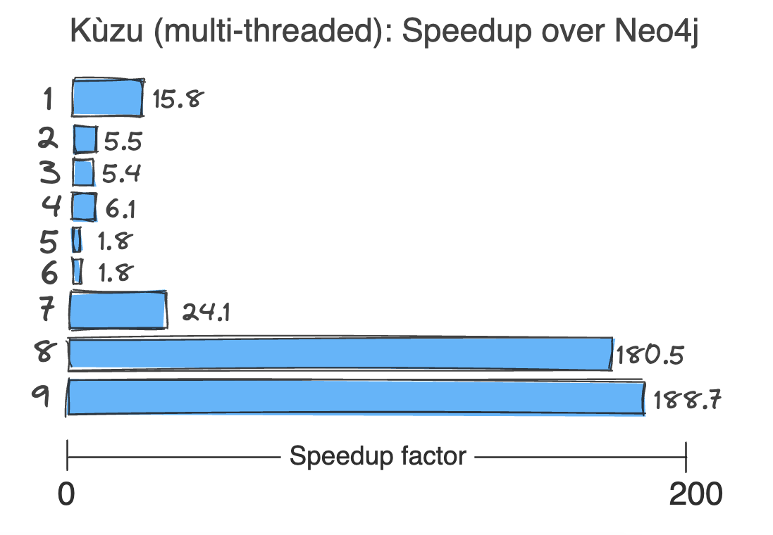
Kùzu’s speedup over Neo4j across 9 queries while running freely on multiple threads 🔥
There are a multitude of reasons why KùzuDB is faster than Neo4j in all queries, and they can be a bit tricky to tease apart. We’ll go through each of them in turn.
Vectorized execution Link to heading
Kùzu executes queries in a vectorized fashion, enabled by the fact that data is stored natively in a column-oriented manner and accessed in batches. This is a similar approach as used by numerous other OLAP DBMSs such as DuckDB3 and ClickHouse4. In modern hardware, column-oriented storage allows better cache utilization, while also allowing CPU optimizations that take advantage of SIMD, a type of parallel processing that performs the same operation on multiple data points via a single instruction.
Multi-threaded execution Link to heading
Query execution is multi-threaded via “morsel-driven parallelism”5 – in this approach, the query workload is divided into several small parts (morsels) that are dynamically distributed between threads during runtime. Each thread takes its own morsel as far through the pipeline as possible, only stopping & synchronizing with other threads when absolutely needed.
Worst-case optimal joins (WCOJ) Link to heading
WCOJ algorithms are a class of join algorithms for queries involving cyclic joins (involving cycles or cliques) over many-to-many relationships in a graph, that are evaluated a column at a time (multi-way), instead of a table at a time (binary). Kùzu generates query plans that seamlessly combine binary joins and WCOJ-style multiway intersections, as described in their blog6. When the query has a strong cyclic component involving many-to-many relationships, WCOJ really speeds up execution, whereas for queries that are more acyclic, binary joins are the go-to.
Factorized execution Link to heading
Factorization is perhaps the most significant contributor to performance, explaining why queries 8 and 9, specifically, show such a huge speedup over Neo4j. Factorization is a compression technique used by query processors to compress intermediate results when evaluating many-to-many joins. This results in an exponential reduction in the ultimate result set size, allowing massive performance gains in queries that involve multi-hop traversals across nodes that possess many-to-many relationships.
Queries 8 and 9 specifically demonstrate the power of factorization, because in this social network graph, finding paths between intermediate nodes can become really expensive at multiple levels of depth due to the presence of “super nodes”, i.e., persons who are followed by thousands of other persons.
Recall that query 9 attempts to find the number of paths to second-degree connections via filters as follows:
MATCH (a:Person)-[r1:Follows]->(b:Person)-[r2:Follows]->(c:Person)
WHERE b.age < 50 AND c.age > 25
RETURN COUNT(*) as numPaths
To analyze what Kùzu’s query planner is doing, we will consider two nodes b of type Person that sit in the middle of the second-degree paths, having 100 incoming edges and 100 outgoing edges. This can be represented graphically as follows.

During query processing, the information that flows between pipeline operators consists of flat tuples, so the graph above will essentially be transformed to sets of redundantly stored tuples with a lot of data repetition. The aim of factorization is to compress this intermediate result set as much as possible, avoiding unnecessary repeated computations at each stage in the query pipeline.
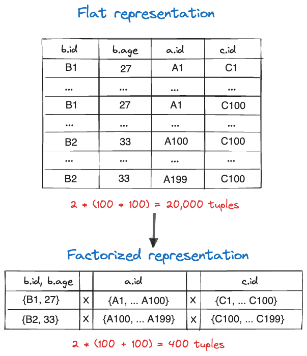
Image inspired by this excellent Kùzu blogpost
As can be seen, the initial flat representation in this simple example had $2 \times (100 \times 100) = 20000$ tuples. However, after factorization, the number of tuples is reduced to $2 \times (100 + 100) = 400$ tuples. This is a 50x reduction in the number of tuples that need to be processed by the query engine, which is already huge. In the real dataset, the data reduction due to factorization is more like 100x, and this only grows as we traverse greater depths in the graph, explaining why these sorts of multi-hop path-finding queries are so much faster in Kùzu than in Neo4j.
Conclusions Link to heading
I hope this post made it clear why KùzuDB is such an exciting graph database. Its embedded nature makes it extremely easy to integrate with existing data workflows, with minimal infrastructure setup. Most importantly, it aims to scale to very large graphs via its key innovations in query processing and performance, which is the main bottleneck in graph analytics today. Another key advantage of embedded databases like Kùzu is the additional reduction in latency due to the fact that queries run within the application layer itself, eliminating the serialization/deserialization overhead of passing blobs of data from a remote server to the application instance.
Even though Kùzu is currently designed to run on a single node only, it follows the DuckDB philosophy of doing the most work possible while utilizing multiple threads and as much memory as is available, so it’s possible to get a lot more done than one might imagine on a single machine. This is a very different approach from Neo4j’s approach to scalability, which uses a “fabric” architecture, requiring far more complex infrastructure, not to mention that it’s a lot more expensive to run.
If you’ve read along this far, you may be wondering, how large of a graph can one analyze in Kùzu? Based on my conversations with the Kùzu team over the last several months, it’s amply clear that Kùzu can scale to graphs that contain hundreds of millions of nodes and billions of edges. In fact, Kùzu is regularly tested on the LDBC-100 graph benchmark, i.e., the 100 Gb variant of this dataset that contains ~280M nodes and 1.7B edges.
I have no doubts that I will be pushing for Kùzu’s use in OLAP-querying large graphs in production, especially for datasets containing many-to-many relationships and a large number of cliques/cycles. The added bonus is that it’s a lot easier for graph data scientists and machine learning practitioners to connect their Kùzu graph to ML libraries like Pytorch Geometric (all it takes is pip install kuzu, without any added infrastructure), so there’s scope for loads more interesting work there!
Thanks for reading this far, and consider going to Kuzu’s GitHub repo, giving them a ⭐️ and showing them some ❤️ on Slack.
Code Link to heading
All the code required to reproduce the results shown in this case study is available on GitHub. I’d love to hear from anybody who uses a similar approach on their own data for even larger graphs, so do reach out if you’ve had success!
Additional resources Link to heading
- Kùzu Slack: Discuss ideas, use cases and issues with the developers and the user community
- Kùzu Blog: Learn about the latest developments and the tool’s internals at a deeper technical level
What every competent graph database management system should do, Kùzu blog ↩︎
RDF support roadmap, KùzuDB GitHub ↩︎
Why DuckDB, DuckDB docs ↩︎
Why is ClickHouse so fast? ClickHouse FAQ ↩︎
Morsel-Driven Parallelism, Leis et al. ↩︎